Systematic literature review

1 Libraries R

Code

library(dplyr)
library(gt)
library(stringr)

2 Loading data R

Code

list_articles <- read.csv2("nlp_full_data_final_18-08-2023.csv", encoding = "UTF-8") %>%
  rename("entry_number" = 1)
list_references <- read.csv2("nlp_references_final_18-08-2023.csv", encoding = "UTF-8") %>%
  rename("citing_art" = 1)
colnames(list_articles) <- gsub("\\.+", "_", colnames(list_articles))
colnames(list_articles) <- gsub("^[[:punct:]]+|[[:punct:]]+$", "", colnames(list_articles))
colnames(list_references) <- gsub("\\.+", "_", colnames(list_references))
colnames(list_references) <- gsub("^[[:punct:]]+|[[:punct:]]+$", "", colnames(list_references))


data_embeddings <- list_articles %>%
  distinct(entry_number, .keep_all = TRUE) %>%
  filter(marketing == 1) %>%
  mutate("year" = substr(prism_coverDate, 7, 10)) %>%
  mutate(keywords = str_replace_all(authkeywords, "\\|", "")) %>%
  mutate(keywords = str_squish(keywords)) %>%
  mutate("combined_text" = paste0(dc_title,". ", dc_description, ". ", keywords))

#write.csv(data_embeddings,"data_for_embeddings.csv")
#data_embeddings <- read.csv("data_for_embeddings.csv")
#embeddings <- read.csv("embeddings_bge.csv")

3 A glimpse of data

Code

data_embeddings %>%
  head(2) %>%
  select(entry_number, dc_creator, combined_text, year) %>%
  gt()

entry_number	dc_creator	combined_text	year
1	Loupos P.	What reviews foretell about opening weekend box office revenue: the harbinger of failure effect in the movie industry. We empirically investigate the harbinger of failure phenomenon in the motion picture industry by analyzing the pre-release reviews written on movies by film critics. We find that harbingers of failure do exist. Their positive (negative) pre-release movie reviews provide a strong predictive signal that the movie will turn out to be a flop (success). This signal persists even for the top critic category, which usually consists of professional critics, indicating that having expertise in a professional domain does not necessarily lead to correct predictions. Our findings challenge the current belief that positive reviews always help enhance box office revenue and shed new light on the influencer-predictor hypothesis. We further analyze the writing style of harbingers and provide new insights into their personality traits and cognitive biases.. Harbingers of failure Movies Preference heterogeneity Reviews Text analytics	2023
2	Krefeld-Schwalb A.	Tighter nets for smaller fishes? Mapping the development of statistical practices in consumer research between 2008 and 2020. During the last decade, confidence in many social sciences, including consumer research, has been undermined by doubts about the replicability of empirical research findings. These doubts have led to increased calls to improve research practices and adopt new measures to increase the replicability of published work from various stakeholders such as funding agencies, journals, and scholars themselves. Despite these demands, it is unclear to which the research published in the leading consumer research journals has adhered to these calls for change. This article provides the first systematic empirical analysis of this question by surveying three crucial statistics of published consumer research over time: sample sizes, effect sizes, and the distribution of published p values. The authors compile a hand-coded sample of N = 258 articles published between 2008 and 2020 in the Journal of Consumer Psychology, the Journal of Consumer Research, and the Journal of Marketing Research. An automated text analysis across all publications in these three journals corroborates the representativeness of the hand-coded sample. Results reveal a substantial increase in sample sizes above and beyond the use of online samples along with a decrease in reported effect sizes. Effect and samples sizes are highly correlated which at least partially explains the reduction in reported effect sizes.. Experimental research methods False-positive results Review	2023

4 Python libraries and loading data

Code

import warnings
warnings.filterwarnings("ignore", message=".*The 'nopython' keyword.*")

import matplotlib.pyplot as plt
import nltk
import numpy as np
import os
import palettable
import pandas as pd
import plotly.express as px
import plotly.io as pio
import string
import stylecloud
import time
import torch
import umap.umap_ as umap


from bertopic import BERTopic
from bertopic.vectorizers import ClassTfidfTransformer
from bertopic.representation import MaximalMarginalRelevance
from gensim.models import Word2Vec
from nltk.corpus import stopwords
from nltk.tokenize import word_tokenize
from palettable import colorbrewer
from sentence_transformers import SentenceTransformer, util
from sklearn.cluster import DBSCAN
from sklearn.decomposition import PCA
from sklearn.feature_extraction.text import CountVectorizer
from sklearn.manifold import TSNE
from sklearn.metrics import davies_bouldin_score, silhouette_score, silhouette_samples
from tabulate import tabulate
from tqdm import tqdm
from transformers import XLNetTokenizer, XLNetModel
from yellowbrick.cluster import SilhouetteVisualizer
from wordcloud import WordCloud



df = pd.read_csv("data_for_embeddings.csv")
#df['title_abstract'] = df['dc_title'].astype(str) + '. ' + df['dc_description'].astype(str)
docs_marketing = df["combined_text"].tolist()

5 CUDA Status and Device Info

Code

print(f"Is CUDA supported by this system? {torch.cuda.is_available()}")

Is CUDA supported by this system? True

Code

print(f"CUDA version: {torch.version.cuda}")

CUDA version: 12.1

Code

# Storing ID of the current CUDA device
cuda_id = torch.cuda.current_device()
print(f"ID of the current CUDA device: {cuda_id}")

ID of the current CUDA device: 0

Code

print(f"Name of the current CUDA device: {torch.cuda.get_device_name(cuda_id)}")

Name of the current CUDA device: NVIDIA GeForce RTX 3070

6 Detect interpretable topics with BERTopic

Note

We use a CountVectorizer which enables us to specify the range of the ngram we want in our topic model. We can use it before or after the topic modelling (update topic).
Here we use it before the topic modelling to exclude english stopwords, but after the embeddings process so that the foundation provided by stopwords in sentences is preserved in context.

6.1 Function to create BERTopics with custom embeddings

The aim of this function is to swiftly create various BERTopic experiments while maintaining the same parameters, except for the choice of the embedding model. This enables the generation of distinct BERTopic results, facilitating meaningful comparisons among them.

Some explanations:

Parameter name	Description
docs	The documents we want to analyze (list).
embeddings_model	Specifies the embeddings model we want to load and use.
min_topic_size	It is used to specify what the minimum size of a topic can be. See BERTopic documentation.
nr_topics	The number of topics we want to reduce our results to. See BERTopic documentation.

Code

def create_bertopic(docs, embeddings_model, min_topic_size, nr_topics):
  
    # initialize a count-based tf-idf transformer
    ctfidf_model = ClassTfidfTransformer(reduce_frequent_words=True)

    # initialize a sentence transformer model for embeddings
    sentence_model = SentenceTransformer(embeddings_model, device='cuda')

    # generate embeddings for the input documents
    embeddings = sentence_model.encode(docs, show_progress_bar=True)
    
    # create the representation model
    #representation_model = MaximalMarginalRelevance(diversity=1)

    # create a bertopic model with specified parameters
    topic_model = BERTopic(
        ctfidf_model=ctfidf_model,
        calculate_probabilities=True,
        verbose=True,
        min_topic_size=min_topic_size,
        nr_topics=nr_topics,
        top_n_words=20
        #representation_model=representation_model
    )

    # fit the bertopic model to the input documents and embeddings
    topics, probs = topic_model.fit_transform(docs, embeddings)

    # update the vectorizer model used by bertopic
    # `min_df` is the minimum document frequency for terms (words or n-grams) in the CountVectorizer.
    updated_vectorizer_model = CountVectorizer(stop_words="english", ngram_range=(1, 3), min_df=3)
    topic_model.update_topics(docs, vectorizer_model=updated_vectorizer_model)

    # return the trained bertopic model
    return topic_model

6.2 Function to visualize BERTopics

Creates a folder in Images/ with the model_name input with various plots in html files.

Code

def generate_topics_table(topic_model):
    # get topic information from the model
    topics_info = topic_model.get_topic_info()

    #  check if topics_info is empty or None
    if topics_info is None or topics_info.empty:
        return "No topics found."

    # convert the data into a list
    data_as_list = topics_info.values.tolist()

    # get column names as headers
    headers = topics_info.columns.tolist()

    # generate the table in HTML format
    table = tabulate(data_as_list, headers, tablefmt='html')

    return table

        

def visualize_bertopic(topic_model, model_name, nr_topics):
    # create the "images" folder if it doesn't exist already
    if not os.path.exists("images"):
        os.makedirs("images")

    # create a subfolder for the specific topic model
    model_folder = os.path.join("images", model_name+"-"+str(nr_topics)+"topics")
    
    # create the model folder if it doesn't exist already
    if not os.path.exists(model_folder):
        os.makedirs(model_folder)
    else:
        # delete existing files in the model folder if it exists
        for file in os.listdir(model_folder):
            os.remove(os.path.join(model_folder, file))

    # generate topics information table
    topics_table = generate_topics_table(topic_model)
    with open(os.path.join(model_folder, 'table_topics.html'), 'w') as f:
        f.write(topics_table)
    
    # visualize topics
    fig_topics = topic_model.visualize_topics()
    fig_topics.write_html(os.path.join(model_folder, "topicsinfo.html"))

    # visualize hierarchy
    fig_hierarchy = topic_model.visualize_hierarchy()
    fig_hierarchy.write_html(os.path.join(model_folder, "hierarchy.html"))

    # visualize hierarchical topics
    hierarchical_topics = topic_model.hierarchical_topics(docs_marketing)
    fig_hierarchical_topics = topic_model.visualize_hierarchy(hierarchical_topics=hierarchical_topics)
    fig_hierarchical_topics.write_html(os.path.join(model_folder, "hierarchical.html"))

    # visualize the bar chart
    fig_barchart = topic_model.visualize_barchart(width=300, height=300, n_words=10, topics=None, top_n_topics=20)
    fig_barchart.write_html(os.path.join(model_folder, "barchart.html"))

    # visualize the heatmap
    fig_heatmap = topic_model.visualize_heatmap()
    fig_heatmap.write_html(os.path.join(model_folder, "heatmap.html"))
    
    # topics over time
    years =  df['year'].to_list()
    topics_over_time = topic_model.topics_over_time(docs_marketing, years)
    fig_topics_over_time = topic_model.visualize_topics_over_time(topics_over_time, top_n_topics=20, normalize_frequency=True)
    fig_topics_over_time.write_html(os.path.join(model_folder, "topicsovertime.html"))

6.3 Create topics for a list of embeddings model

We must specify the number of topics we want to create (nbtopics) and the minimum number of documents to form a topic (nbmintopicsize).

Code

#09/26/2023 -----------------------------------------
#to-do  clean code : embeddings are charged twice for viz purposes (document viz) because it is loaded a first time in the create_bertopic function and again in the loop (can't use just the model name in visualize_bertopic function.)
#---------------------------------------------------

# list of embeddings models
list_embeddings = ["all-mpnet-base-v2"]
#list_embeddings = ["all-mpnet-base-v2","multi-qa-mpnet-base-dot-v1","all-roberta-large-v1","all-MiniLM-L12-v2"]

# create a list to store model information
table_data = []
topic_models = {}
#nbtopics is the number of topics we want to create/reduce to
#nbmintopicsize is the minimum number of documents to form a topic
nbtopics = 17
nbmintopicsize = 5


# loop through the list of embeddings models and create topic_model + viz in images
for embeddings_model in list_embeddings:
    print(f"\nCreating BERTopics with the {embeddings_model} Sentence-Transformers pretrained model.")
    topic_model = create_bertopic(docs_marketing, embeddings_model, nbmintopicsize, nbtopics)
    print(f"\nCreating BERTopic visualizations in the `images\\{embeddings_model}-{nbtopics}topics` folder.")
    visualize_bertopic(topic_model, embeddings_model, nbtopics)
    chargedmodel = SentenceTransformer(embeddings_model, device='cuda')
    
     # visualize the documents
    model_folder = os.path.join("images", embeddings_model+"-"+str(nbtopics)+"topics")
    embeddings = chargedmodel.encode(docs_marketing, show_progress_bar=False)
    fig_documents = topic_model.visualize_documents(docs_marketing, embeddings=embeddings)
    fig_documents.write_html(os.path.join(model_folder, "documents_topics.html"))
    
    # to summarize embeddings' models
    dimensions =  chargedmodel.get_sentence_embedding_dimension()
    max_tokens = chargedmodel.max_seq_length
    # store the topic_model in the dictionary with the embeddings name as key
    topic_models[embeddings_model] = topic_model
    # add model information to the table data list
    table_data.append([embeddings_model, dimensions, max_tokens])


Creating BERTopics with the all-mpnet-base-v2 Sentence-Transformers pretrained model.

Creating BERTopic visualizations in the `images\all-mpnet-base-v2-17topics` folder.


Batches:   0%|          | 0/13 [00:00<?, ?it/s]
Batches:   8%|7         | 1/13 [00:00<00:09,  1.29it/s]
Batches:  15%|#5        | 2/13 [00:01<00:07,  1.49it/s]
Batches:  23%|##3       | 3/13 [00:01<00:06,  1.67it/s]
Batches:  31%|###       | 4/13 [00:02<00:05,  1.78it/s]
Batches:  38%|###8      | 5/13 [00:02<00:04,  1.94it/s]
Batches:  46%|####6     | 6/13 [00:02<00:03,  2.04it/s]
Batches:  54%|#####3    | 7/13 [00:03<00:02,  2.29it/s]
Batches:  62%|######1   | 8/13 [00:03<00:01,  2.66it/s]
Batches:  69%|######9   | 9/13 [00:03<00:01,  3.08it/s]
Batches:  77%|#######6  | 10/13 [00:03<00:00,  3.47it/s]
Batches:  85%|########4 | 11/13 [00:04<00:00,  3.86it/s]
Batches:  92%|#########2| 12/13 [00:04<00:00,  4.46it/s]
Batches: 100%|##########| 13/13 [00:04<00:00,  3.01it/s]
2023-10-04 17:06:54,764 - BERTopic - Reduced dimensionality
2023-10-04 17:06:54,798 - BERTopic - Clustered reduced embeddings
2023-10-04 17:06:55,034 - BERTopic - Reduced number of topics from 18 to 17

  0%|          | 0/15 [00:00<?, ?it/s]
100%|##########| 15/15 [00:00<00:00, 295.69it/s]

0it [00:00, ?it/s]
14it [00:00, 129.70it/s]
19it [00:00, 79.92it/s] 
21it [00:00, 69.00it/s]

Code

# table headers
headers = ["Embeddings Model", "Dimensions", "Max Tokens"]

# title for the table, centered
table_title = "Summary of Embeddings Models used"

# create the table with centered title
table = tabulate(table_data, headers, tablefmt="pretty")
table_lines = table.split("\n")
table_lines.insert(0, table_title.center(len(table_lines[0])))
table_with_centered_title = "\n".join(table_lines)

# display the table with centered title
print("\n")

Code

print(table_with_centered_title)

       Summary of Embeddings Models used       
+-------------------+------------+------------+
| Embeddings Model  | Dimensions | Max Tokens |
+-------------------+------------+------------+
| all-mpnet-base-v2 |    768     |    384     |
+-------------------+------------+------------+

Code


#sentence_model.max_seq_length
#sentence_model.get_sentence_embedding_dimension()

7 Topics Results

7.1 Representative documents of topics

Code

# we can access the different topic models like this
embeddings_model_name = "all-mpnet-base-v2"
topics_list = topic_models[embeddings_model_name].topics_


# len(topic_models[embeddings_model_name].probabilities_) # = 405 like the docs_marketings
# len(topic_models[embeddings_model_name].topics_)        # = 405 like the docs_marketings
# type(topic_models[embeddings_model_name].topics_)      # list

# put the topics' number in the df of marketing documents
df["topic"] = topics_list

# get the correspondence between topic number and topic name
topic_info_df = topic_models[embeddings_model_name].get_topic_info()

selected_columns = topic_info_df[["Topic", "Name"]]

topic_info_df

    Topic  ...                                Representative_Docs
0      -1  ...  [An Artificial Intelligence Method for the Ana...
1       0  ...  [Differences in Online Review Content between ...
2       1  ...  [Young People Under ‘Finfluencer’: The Rise of...
3       2  ...  [A Scientometric Analysis of Publications in t...
4       3  ...  [Building a sustainable brand image in luxury ...
5       4  ...  [A machine-learning based approach to measurin...
6       5  ...  [What’s yours is mine: exploring customer voic...
7       6  ...  [Should We Continue Using Intelligent Virtual ...
8       7  ...  [Using text mining to track changes in travel ...
9       8  ...  [Automated marketing research using online cus...
10      9  ...  [Deep Learning Applications for Interactive Ma...
11     10  ...  [Exploring mobile banking service quality dime...
12     11  ...  [Disclosure of Brand-Related Information and F...
13     12  ...  [Exploring customer concerns on service qualit...
14     13  ...  [Wordify: A Tool for Discovering and Different...
15     14  ...  [Understanding retail quality of sporting good...
16     15  ...  [Using AI predicted personality to enhance adv...

[17 rows x 5 columns]

7.2 Distribution of topics

Code

df["topic_name"] = df["topic"].map(selected_columns.set_index("Topic")["Name"])

# Calculate the count and percentage of each topic
topic_counts = df["topic_name"].value_counts().reset_index()
topic_counts.columns = ["topic_name", "count"]
topic_counts["percentage"] = (topic_counts["count"] / sum(topic_counts['count'])) * 100

# Add "(outliers)" to the name of the first topic of topic_counts
topic_counts.iloc[0, 0] = "<b>(outliers)</b> " + topic_counts.iloc[0, 0]

if 'figdistrib' not in globals():
    figdistrib = px.bar(topic_counts, x="topic_name", y="percentage", title="Distribution of Topics Among Articles",
                        hover_data=["count"])
    figdistrib.update_layout(template="plotly_white")
    # Some aesthetics on the graph
    figdistrib.update_xaxes(title_text="BERTopics")
    figdistrib.update_yaxes(title_text="Percentage of articles")
    figdistrib.update_traces(marker_color="rgb(158,202,225)", marker_line_color="rgb(8,48,107)", marker_line_width=1.5, opacity=0.6)
    figdistrib.update_layout(title_x=0.5, title_xanchor="center")

Code


#figdistrib.show()

7.3 Distribution of topics without outliers

Code

# Creates dataframe from Series
topic_counts_no_outliers = df["topic_name"].value_counts().reset_index()

# Excluding the first row (outliers) from topic_counts
topic_counts_no_outliers = topic_counts_no_outliers.iloc[1:]

# Calculate the count and percentage of each topic without considering outliers
topic_counts_no_outliers.columns = ["topic_name", "count"]
topic_counts_no_outliers["percentage"] = (topic_counts_no_outliers["count"] / sum(topic_counts_no_outliers['count'])) * 100



if 'figdistrib2' not in globals():
    figdistrib2 = px.bar(topic_counts_no_outliers, x="topic_name", y="percentage", title="Distribution of Topics Among Articles",
                        hover_data=["count"])
    figdistrib2.update_layout(template="plotly_white")
    # Some aesthetics on the graph
    figdistrib2.update_xaxes(title_text="BERTopics")
    figdistrib2.update_yaxes(title_text="Percentage of articles")
    figdistrib2.update_traces(marker_color="rgb(158,202,225)", marker_line_color="rgb(8,48,107)", marker_line_width=1.5, opacity=0.6)
    figdistrib2.update_layout(title_x=0.5, title_xanchor="center")

Code


#figdistrib.show()

7.4 Visualize how each token contributes to a specific topic.

We can do it by selecting a sentence in the document. To do so, we need to first calculate topic distributions on a token level and then visualize the results:
More parameters here :
https://maartengr.github.io/BERTopic/getting_started/distribution/distribution.html

Here, we take the most cited article as an example.

Code

# Calculate the topic distributions on a token-level for the all-mpnet-base-v2 model, we can add the window
topic_distr, topic_token_distr = topic_models["all-mpnet-base-v2"].approximate_distribution(docs_marketing, calculate_tokens=True)


  0%|          | 0/1 [00:00<?, ?it/s]
100%|##########| 1/1 [00:01<00:00,  1.26s/it]

Code

# Visualize the token-level distributions, put id of document
df_topicmodel = topic_models["all-mpnet-base-v2"].visualize_approximate_distribution(docs_marketing[382], topic_token_distr[382])
df_topicmodel

	Mine	your	own	business	Market	structure	surveillance	through	text	mining	Web	provides	gathering	of	data	regarding	consumers	experiences	and	even	interactions	an	approach	for	firms	to	explore	online	user	content	and	listen	to	what	customers	to	convert	the	user	in	obtaining	such	market	structure	insights	from	online	user	content	is	that	consumers	employ	text	mining	approach	and	combine	with	semantic	network	analysis	tools	drugs	generating	market	structure	perceptual	maps	consumer	We	compare	market	structure	based	on	user	content	data	with	market	structure	derived	from	and	survey	based	data	to	establish	validity	INFORMS	Market	structure	Marketing	research	Text	mining	User	generated
0_reviews_online_review_product	0.000	0.000	0.000	0.000	0.000	0.000	0.125	0.125	0.125	0.125	0.000	0.000	0.000	0.000	0.000	0.000	0.000	0.000	0.000	0.000	0.000	0.000	0.000	0.000	0.000	0.000	0.000	0.000	0.000	0.120	0.120	0.120	0.120	0.000	0.000	0.000	0.000	0.000	0.000	0.000	0.000	0.000	0.000	0.106	0.209	0.209	0.209	0.103	0.167	0.167	0.167	0.167	0.000	0.000	0.000	0.000	0.000	0.000	0.000	0.000	0.000	0.000	0.000	0.000	0.000	0.000	0.000	0.000	0.000	0.000	0.000	0.000	0.000	0.000	0.000	0.000	0.000	0.000	0.000	0.000	0.000	0.000	0.000	0.000	0.000	0.000	0.000	0.000	0.000	0.000	0.000	0.000	0.000	0.000	0.000	0.000	0.000	0.000	0.000	0.000
1_engagement_media_social media_social	0.000	0.000	0.000	0.000	0.000	0.000	0.000	0.112	0.213	0.213	0.213	0.100	0.000	0.000	0.000	0.000	0.000	0.000	0.000	0.000	0.000	0.000	0.000	0.000	0.000	0.000	0.000	0.000	0.000	0.143	0.143	0.143	0.143	0.000	0.000	0.000	0.000	0.000	0.000	0.000	0.000	0.000	0.000	0.000	0.000	0.000	0.000	0.000	0.190	0.190	0.190	0.190	0.000	0.000	0.000	0.000	0.000	0.000	0.000	0.000	0.000	0.000	0.000	0.000	0.000	0.000	0.000	0.000	0.000	0.000	0.000	0.000	0.000	0.000	0.000	0.000	0.000	0.000	0.000	0.000	0.000	0.000	0.000	0.000	0.000	0.000	0.000	0.000	0.000	0.000	0.000	0.000	0.000	0.000	0.000	0.000	0.000	0.000	0.000	0.000
2_research_marketing_journal_consumer	0.126	0.247	0.247	0.247	0.121	0.000	0.158	0.281	0.409	0.409	0.251	0.128	0.000	0.000	0.000	0.000	0.000	0.000	0.000	0.000	0.000	0.000	0.000	0.000	0.000	0.000	0.000	0.000	0.000	0.000	0.000	0.000	0.000	0.000	0.000	0.000	0.000	0.000	0.000	0.000	0.000	0.000	0.000	0.000	0.000	0.000	0.000	0.000	0.000	0.000	0.000	0.000	0.000	0.000	0.000	0.000	0.000	0.000	0.000	0.000	0.000	0.000	0.000	0.000	0.000	0.000	0.000	0.000	0.000	0.000	0.000	0.000	0.000	0.000	0.000	0.000	0.000	0.000	0.000	0.000	0.000	0.000	0.000	0.000	0.000	0.000	0.000	0.000	0.000	0.000	0.000	0.000	0.166	0.343	0.530	0.530	0.364	0.187	0.000	0.000
3_brand_luxury_fashion_brands	0.000	0.000	0.000	0.000	0.000	0.000	0.147	0.262	0.366	0.366	0.219	0.104	0.000	0.000	0.000	0.000	0.000	0.000	0.000	0.000	0.000	0.000	0.000	0.000	0.000	0.000	0.000	0.000	0.000	0.000	0.000	0.000	0.000	0.000	0.000	0.000	0.000	0.000	0.000	0.000	0.000	0.000	0.000	0.000	0.000	0.000	0.000	0.000	0.102	0.102	0.102	0.102	0.000	0.116	0.116	0.116	0.116	0.000	0.000	0.000	0.000	0.000	0.000	0.000	0.000	0.000	0.000	0.000	0.000	0.000	0.000	0.000	0.000	0.000	0.000	0.000	0.000	0.110	0.110	0.110	0.110	0.000	0.000	0.000	0.000	0.000	0.000	0.000	0.000	0.000	0.000	0.000	0.000	0.000	0.000	0.000	0.000	0.000	0.000	0.000
4_marketing_data_text_analysis	0.000	0.000	0.000	0.000	0.000	0.127	0.372	0.553	0.731	0.604	0.360	0.178	0.000	0.116	0.116	0.116	0.116	0.000	0.000	0.000	0.000	0.000	0.000	0.000	0.000	0.000	0.000	0.000	0.000	0.000	0.000	0.000	0.000	0.000	0.000	0.000	0.000	0.000	0.000	0.000	0.000	0.000	0.000	0.000	0.000	0.000	0.000	0.000	0.000	0.000	0.000	0.000	0.000	0.137	0.137	0.137	0.137	0.000	0.117	0.236	0.236	0.236	0.119	0.000	0.000	0.000	0.000	0.000	0.000	0.000	0.000	0.000	0.000	0.000	0.000	0.000	0.000	0.201	0.304	0.304	0.304	0.103	0.000	0.000	0.135	0.271	0.374	0.482	0.347	0.211	0.108	0.000	0.122	0.285	0.456	0.456	0.333	0.171	0.000	0.000
5_hotel_service_reviews_online	0.000	0.000	0.000	0.000	0.000	0.000	0.137	0.241	0.345	0.345	0.208	0.103	0.000	0.000	0.000	0.000	0.000	0.112	0.112	0.112	0.112	0.000	0.000	0.000	0.000	0.000	0.000	0.000	0.000	0.000	0.000	0.124	0.124	0.124	0.124	0.000	0.000	0.000	0.000	0.000	0.000	0.000	0.000	0.000	0.106	0.106	0.106	0.106	0.000	0.000	0.000	0.000	0.000	0.101	0.101	0.101	0.101	0.000	0.000	0.000	0.000	0.000	0.000	0.000	0.000	0.000	0.000	0.000	0.000	0.000	0.000	0.000	0.000	0.000	0.000	0.000	0.000	0.000	0.000	0.000	0.000	0.000	0.000	0.000	0.000	0.000	0.000	0.000	0.000	0.000	0.000	0.000	0.000	0.000	0.000	0.000	0.000	0.000	0.000	0.000
6_ai_intelligence_artificial_artificial intelligence	0.000	0.000	0.000	0.000	0.000	0.000	0.000	0.000	0.000	0.000	0.000	0.000	0.000	0.000	0.000	0.000	0.000	0.000	0.000	0.000	0.000	0.000	0.000	0.000	0.000	0.000	0.000	0.000	0.000	0.000	0.000	0.000	0.000	0.000	0.000	0.000	0.000	0.000	0.000	0.000	0.000	0.000	0.000	0.000	0.000	0.000	0.000	0.000	0.101	0.101	0.101	0.101	0.000	0.000	0.000	0.000	0.000	0.000	0.000	0.000	0.000	0.000	0.000	0.000	0.000	0.000	0.000	0.000	0.000	0.000	0.000	0.000	0.000	0.000	0.000	0.000	0.000	0.000	0.000	0.000	0.000	0.000	0.000	0.000	0.000	0.000	0.000	0.000	0.000	0.000	0.000	0.000	0.000	0.000	0.000	0.000	0.000	0.000	0.000	0.000
7_tourism_destination_tourists_destinations	0.000	0.000	0.000	0.000	0.000	0.000	0.137	0.281	0.410	0.410	0.273	0.129	0.000	0.000	0.000	0.000	0.000	0.000	0.000	0.000	0.000	0.000	0.000	0.000	0.000	0.000	0.000	0.000	0.000	0.000	0.000	0.000	0.000	0.000	0.000	0.000	0.000	0.000	0.000	0.000	0.000	0.000	0.000	0.000	0.000	0.000	0.000	0.000	0.000	0.000	0.000	0.000	0.000	0.000	0.000	0.000	0.000	0.000	0.000	0.000	0.000	0.000	0.000	0.000	0.000	0.000	0.000	0.000	0.000	0.000	0.000	0.000	0.000	0.000	0.000	0.000	0.000	0.000	0.000	0.000	0.000	0.000	0.000	0.000	0.000	0.000	0.000	0.000	0.000	0.000	0.000	0.000	0.000	0.000	0.000	0.000	0.000	0.000	0.000	0.000
8_product_reviews_analysis_online	0.000	0.129	0.277	0.425	0.565	0.553	0.616	0.623	0.627	0.510	0.300	0.145	0.000	0.000	0.000	0.000	0.000	0.000	0.000	0.000	0.000	0.000	0.000	0.000	0.000	0.106	0.106	0.106	0.106	0.000	0.000	0.000	0.000	0.000	0.000	0.000	0.000	0.000	0.000	0.137	0.277	0.432	0.586	0.596	0.613	0.459	0.305	0.158	0.000	0.000	0.000	0.000	0.000	0.111	0.111	0.111	0.111	0.000	0.000	0.000	0.000	0.000	0.000	0.114	0.218	0.331	0.331	0.217	0.113	0.136	0.270	0.412	0.562	0.540	0.407	0.264	0.115	0.158	0.313	0.438	0.563	0.405	0.250	0.125	0.000	0.000	0.000	0.000	0.000	0.000	0.000	0.125	0.301	0.430	0.574	0.584	0.525	0.396	0.252	0.117
9_learning_deep_deep learning_models	0.000	0.000	0.000	0.000	0.000	0.000	0.000	0.000	0.000	0.000	0.000	0.000	0.000	0.000	0.000	0.000	0.000	0.000	0.000	0.000	0.000	0.000	0.000	0.000	0.000	0.000	0.000	0.000	0.000	0.112	0.112	0.112	0.112	0.000	0.000	0.000	0.000	0.000	0.000	0.000	0.000	0.000	0.000	0.000	0.000	0.000	0.000	0.000	0.128	0.128	0.128	0.128	0.000	0.000	0.000	0.000	0.000	0.000	0.000	0.000	0.000	0.000	0.000	0.000	0.000	0.000	0.000	0.000	0.000	0.000	0.000	0.000	0.000	0.000	0.000	0.000	0.000	0.115	0.115	0.115	0.115	0.000	0.000	0.000	0.000	0.000	0.000	0.000	0.000	0.000	0.000	0.000	0.000	0.000	0.000	0.000	0.000	0.000	0.000	0.000
10_mobile_customer_quality_banking	0.000	0.000	0.000	0.000	0.000	0.000	0.183	0.331	0.472	0.472	0.288	0.141	0.000	0.000	0.000	0.000	0.000	0.000	0.000	0.000	0.000	0.000	0.000	0.000	0.000	0.116	0.116	0.116	0.116	0.000	0.000	0.137	0.137	0.137	0.137	0.116	0.116	0.116	0.116	0.000	0.000	0.000	0.000	0.000	0.133	0.133	0.133	0.133	0.000	0.000	0.000	0.000	0.141	0.326	0.326	0.326	0.185	0.000	0.000	0.000	0.000	0.000	0.000	0.000	0.000	0.000	0.000	0.000	0.000	0.000	0.000	0.000	0.000	0.000	0.000	0.000	0.000	0.000	0.000	0.000	0.000	0.000	0.000	0.000	0.000	0.000	0.000	0.000	0.000	0.000	0.000	0.000	0.000	0.000	0.000	0.000	0.000	0.000	0.000	0.000
11_firm_financial_firms_investment	0.000	0.000	0.000	0.000	0.000	0.000	0.000	0.000	0.000	0.000	0.000	0.000	0.000	0.000	0.000	0.000	0.000	0.000	0.000	0.000	0.000	0.185	0.370	0.541	0.703	0.518	0.333	0.162	0.000	0.000	0.000	0.000	0.000	0.000	0.000	0.000	0.000	0.000	0.000	0.000	0.000	0.000	0.000	0.000	0.000	0.000	0.000	0.000	0.000	0.000	0.000	0.000	0.000	0.000	0.000	0.000	0.000	0.000	0.000	0.000	0.000	0.000	0.000	0.000	0.000	0.000	0.000	0.000	0.000	0.000	0.000	0.000	0.000	0.000	0.000	0.000	0.000	0.000	0.000	0.000	0.000	0.000	0.000	0.000	0.000	0.000	0.000	0.000	0.000	0.000	0.000	0.000	0.000	0.000	0.000	0.000	0.000	0.000	0.000	0.000
12_covid19_crisis_pandemic_social	0.000	0.000	0.000	0.000	0.000	0.000	0.115	0.115	0.115	0.115	0.000	0.000	0.000	0.000	0.000	0.000	0.000	0.000	0.000	0.000	0.000	0.000	0.000	0.000	0.000	0.000	0.000	0.000	0.000	0.000	0.000	0.000	0.000	0.000	0.000	0.000	0.000	0.000	0.000	0.000	0.000	0.000	0.000	0.000	0.000	0.000	0.000	0.000	0.000	0.000	0.000	0.000	0.000	0.000	0.000	0.000	0.000	0.000	0.000	0.000	0.000	0.000	0.000	0.000	0.000	0.000	0.000	0.000	0.000	0.000	0.000	0.000	0.000	0.000	0.000	0.000	0.000	0.000	0.000	0.000	0.000	0.000	0.000	0.000	0.000	0.000	0.000	0.000	0.000	0.000	0.000	0.000	0.000	0.000	0.000	0.000	0.000	0.000	0.000	0.000
13_sentiment_text_voice_social	0.000	0.000	0.000	0.000	0.000	0.000	0.104	0.104	0.104	0.104	0.000	0.000	0.000	0.000	0.000	0.000	0.000	0.000	0.000	0.000	0.000	0.000	0.000	0.000	0.000	0.000	0.000	0.000	0.000	0.000	0.000	0.000	0.000	0.000	0.000	0.000	0.000	0.000	0.000	0.000	0.000	0.000	0.000	0.000	0.000	0.000	0.000	0.000	0.000	0.000	0.000	0.000	0.000	0.000	0.000	0.000	0.000	0.000	0.000	0.000	0.000	0.000	0.000	0.000	0.000	0.000	0.000	0.000	0.000	0.000	0.000	0.000	0.000	0.000	0.000	0.000	0.000	0.000	0.000	0.000	0.000	0.000	0.000	0.000	0.000	0.000	0.000	0.000	0.000	0.000	0.000	0.000	0.000	0.000	0.000	0.000	0.000	0.000	0.000	0.000
14_retail_value_goods_dimensions	0.000	0.000	0.000	0.000	0.000	0.000	0.184	0.381	0.561	0.698	0.514	0.317	0.137	0.000	0.000	0.000	0.000	0.000	0.000	0.000	0.000	0.000	0.000	0.000	0.000	0.000	0.000	0.000	0.000	0.000	0.000	0.000	0.000	0.000	0.000	0.000	0.000	0.000	0.000	0.000	0.000	0.000	0.000	0.000	0.000	0.000	0.000	0.000	0.000	0.000	0.000	0.000	0.157	0.387	0.522	0.522	0.365	0.135	0.000	0.000	0.000	0.000	0.000	0.000	0.000	0.000	0.000	0.000	0.000	0.000	0.000	0.000	0.000	0.000	0.000	0.000	0.000	0.000	0.000	0.000	0.000	0.000	0.000	0.000	0.000	0.000	0.000	0.000	0.000	0.000	0.000	0.000	0.000	0.000	0.000	0.000	0.000	0.000	0.000	0.000

Code

topics_html = df_topicmodel.to_html()

with open('images/topics_contribution.html', 'w') as html_file:
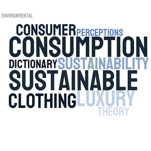
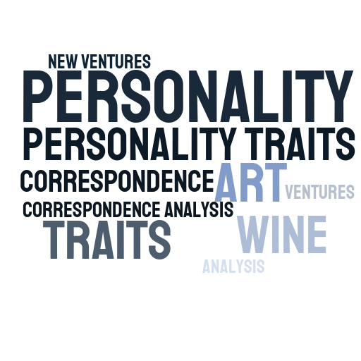
    html_file.write(topics_html)

7.5 Some visualizations of the topics

7.6 Wordclouds of BERTopics

Code

from wordcloud import WordCloud

def create_wordcloud_text(model, topic):
    text = {word.upper(): value for word, value in topic_model.get_topic(topic)}
    return text


text = create_wordcloud_text(topic_model, 0)

Code

# A lot of palettes available here: https://jiffyclub.github.io/palettable/
import os
from tqdm import tqdm
import stylecloud

# Set the full path to the output folder
output_folder = "wordclouds"

# Make sure the output folder exists, or create it if it doesn't
if not os.path.exists(output_folder):
    os.makedirs(output_folder)

palettes = [
    ('wesanderson.GrandBudapest2_4', 'GrandBudapest2_4')
    #('scientific.sequential.Oslo_10', 'Oslo_10'),
    #('scientific.sequential.GrayC_10', 'GrayC_10'),
    #('scientific.sequential.GrayC_4', 'GrayC_4'),
    #('scientific.sequential.GrayC_5', 'GrayC_5'),
    #('scientific.sequential.GrayC_6', 'GrayC_6'),
    #('scientific.sequential.GrayC_3', 'GrayC_3'),
    #('colorbrewer.sequential.Blues_9', 'Blues_9'),
    #('colorbrewer.sequential.BuGn_9', 'BuGn_9'),
    #('colorbrewer.sequential.BuPu_9', 'BuPu_9'),
    #('colorbrewer.sequential.GnBu_9', 'GnBu_9'),
    #('colorbrewer.sequential.OrRd_9', 'OrRd_9'),
    #('colorbrewer.sequential.Oranges_9', 'Oranges_9'),
    #('colorbrewer.sequential.PuRd_9', 'PuRd_9'),
    #('colorbrewer.sequential.YlOrRd_9', 'YlOrRd_9'),
    #('wesanderson.GrandBudapest3_6', 'GrandBudapest3_6'),
    #('wesanderson.Moonrise7_5', 'Moonrise7_5'),
    #('wesanderson.Zissou_5', 'Zissou_5'),
    #('scientific.sequential.Bilbao_10', 'Bilbao_10')
]

# Define the number of topics
nb_topics = len(topic_model.get_topic_info()) - 1  # Exclude topic -1 (outliers from BERTopic)

# Loop through topics and palettes
for palette, palette_name in palettes:
    # Create a progress bar for the current palette
    progress_bar = tqdm(total=nb_topics, desc=f"Palette: {palette_name}", position=0, leave=True)
    
    for i in range(0, nb_topics):
        text = create_wordcloud_text(model=topic_model, topic=i)
        try:
            # Generate the word cloud with the specified palette and save it in the "wordclouds" folder
            output_name = os.path.join(output_folder, f'wordcloud_topic{i}_{palette_name}.png')
            stylecloud.gen_stylecloud(text=text,
                                      palette=palette, background_color='white',
                                      size=512,
                                      gradient='radial', output_name=output_name, collocations=True)
        except AttributeError:
            print(f"Palette {palette_name} does not exist.")
        
        # Update the progress bar for the current palette
        progress_bar.update(1)
    
    # Close the progress bar for the current palette
    progress_bar.close()

Code

print("\nAll word clouds have been generated in the 'wordclouds' folder.")


All word clouds have been generated in the 'wordclouds' folder.

7.6.1 Wordcloud using the Scientific - Sequential - Oslo_10 color palette

More to see here: Grid wordclouds

Topic 0	Topic 1	Topic 2	Topic 3

Topic 4	Topic 5	Topic 6	Topic 7

Topic 8	Topic 9	Topic 10	Topic 11

Topic 12	Topic 13	Topic 14	Topic 15

8 BERTopic with Custom Embeddings model (xlnet)

(Yang et al. (2019))

9 Word2Vec model (tokenization with nltk)

Code


# Define your Word2Vec parameters
vector_size = 300   # Set the embedding vector size
window_size = 15   # Define the context window size
min_count = 5     # Ignore words with a frequency below min_count
sg = 1             # Use CBOW (or skip-gram if sg=1)

# Function to check if a word is a string (excluding numbers)
def is_string(word):
    return isinstance(word, str) and not any(char.isdigit() for char in word)

# Load NLTK stopwords
stop_words = set(stopwords.words("english"))

# tokenize the marketing documents into sentences, convert to lowercase, remove stopwords,
# remove punctuation, and keep only words made of letters
def preprocess_text(text):
    tokens = word_tokenize(text)
    filtered_tokens = [
        word.lower()
        for word in tokens
        if is_string(word)
        and word.lower() not in stop_words
        and word not in string.punctuation
        and word.isalpha()  # Check if the word contains only letters
    ]
    return filtered_tokens

tokenized_docs_marketing = [preprocess_text(sentence) for sentence in docs_marketing]

# train the Word2Vec model
model = Word2Vec(
    tokenized_docs_marketing, 
    vector_size=vector_size, 
    window=window_size, 
    min_count=min_count, 
    sg=sg
)

similar_words = model.wv.most_similar("learning", topn=20)
similar_words_df = pd.DataFrame(similar_words, columns=['Word', 'Similarity score'])
df_similar_words = pd.DataFrame(similar_words_df)

#df_similar_words

9.1 Plot similar words for “learning”

Code

# Plot graph with Plotly Express
if 'figlearning' not in globals():
    figlearning = px.scatter(similar_words_df, x='Similarity score', y='Word', color='Word',
                     title='Top 20 Most Similar Words for "learning"')
    
    # Customize the style of the plot
    figlearning.update_traces(marker=dict(size=12, opacity=0.6),
                      selector=dict(mode='markers'),
                      showlegend=False)
    
    figlearning.update_layout(title_x=0.5, title_font=dict(size=20))
    figlearning.update_layout(template="plotly_white")

Code


# Show the plot
#figlearning.show()

# Save the plot as an HTML file
figlearning.write_html("similar_words_plot.html")

9.2 Plot Word2Vec embeddings in 3D with plotly

The visualization is quite heavy so it’s not displayed here but you can find it here: visualization

Code

# Extract word vectors and corresponding words from the Word2Vec model
word_vectors = [model.wv[word] for word in model.wv.index_to_key]
words = model.wv.index_to_key
#len(words) => 2122 words and vectors

# Convert word_vectors to a NumPy array
word_vectors_array = np.array(word_vectors)

# Perform t-SNE to reduce the word vectors to 3D
tsne = TSNE(n_components=3, perplexity=30, learning_rate=200, n_iter=500, random_state=42, verbose=1)
tsne_result = tsne.fit_transform(word_vectors_array)

[t-SNE] Computing 91 nearest neighbors...
[t-SNE] Indexed 2122 samples in 0.001s...
[t-SNE] Computed neighbors for 2122 samples in 0.271s...
[t-SNE] Computed conditional probabilities for sample 1000 / 2122
[t-SNE] Computed conditional probabilities for sample 2000 / 2122
[t-SNE] Computed conditional probabilities for sample 2122 / 2122
[t-SNE] Mean sigma: 0.144301
[t-SNE] KL divergence after 250 iterations with early exaggeration: 74.836838
[t-SNE] KL divergence after 500 iterations: 1.318700

Code


# Create a DataFrame with the reduced dimensions and words
tsne_df = pd.DataFrame({'Word': words, 'Dimension 1': tsne_result[:, 0], 'Dimension 2': tsne_result[:, 1], 'Dimension 3': tsne_result[:, 2]})

# Check if the rendering has already been done
if 'figlearning' not in globals():
    # Rendering code (this will only be executed once)
    
    # Create a 3D scatter plot with Plotly Express
    fig3D = px.scatter_3d(tsne_df, x='Dimension 1', y='Dimension 2', z='Dimension 3', text='Word', title='3D Word Embedding Visualization')

    # Customize the style of the plot
    fig3D.update_traces(marker=dict(size=6, opacity=0.6),
                      selector=dict(mode='markers+text'))

    fig3D.update_layout(title_x=0.5, title_font=dict(size=20))
    fig3D.update_layout(template="plotly_white")
    
    # Save the plot as an HTML file
    fig3D.write_html("word2vec_embeddings_3d_plot.html")
    
# Show the plot
#fig.show()

9.3 Plot Word2Vec embeddings in 2D with plotly

Code

# Calculate word frequencies in text data
word_frequencies = {}  # Dictionary to store word frequencies
for sentence in tokenized_docs_marketing:
    for word in sentence:
        if word in word_frequencies:
            word_frequencies[word] += 1
        else:
            word_frequencies[word] = 1

# Create a DataFrame with the reduced dimensions, words, and frequencies
tsne_df = pd.DataFrame({'Word': words, 'Dimension 1': tsne_result[:, 0], 'Dimension 2': tsne_result[:, 1]})

# Add a new column for word frequencies
tsne_df['Frequency'] = tsne_df['Word'].apply(lambda word: word_frequencies.get(word, 1))

if 'figw2v' not in globals():
    # Rendering code (this will only be executed once)
    # Create a 2D scatter plot with Plotly Express
    figw2v = px.scatter(
        tsne_df,
        x='Dimension 1',
        y='Dimension 2',
        text='Word',
        title='2D Word Embedding Visualization with Point Size based on Frequency',
        size_max=50,  # Set the maximum size of words
        size='Frequency',
        color_discrete_sequence=['blue'],# Use raw frequency for text size
    )
    
    # Customize the style of the plot
    figw2v.update_traces(opacity=0.6)
    
    figw2v.update_layout(title_x=0.5, title_font=dict(size=20))
    figw2v.update_layout(template="plotly_white")

Code


# Show the plot
#figw2v.show()

# Save the plot as an HTML file
figw2v.write_html("word2vec_embeddings_2d_plot.html")

10 Plotting authors and text based on BERTopic

10.1 3D plot of authors (t-SNE + BERTopic clustering)

The visualization is quite heavy so it’s not displayed here but you can find it here: visualization

Code

# Step 1: Perform t-SNE dimensionality reduction on word vectors to 3D
tsne = TSNE(n_components=3, perplexity=30, learning_rate=200, n_iter=1337, random_state=42, verbose=1)
tsne_result = tsne.fit_transform(embeddings)

[t-SNE] Computing 91 nearest neighbors...
[t-SNE] Indexed 405 samples in 0.001s...
[t-SNE] Computed neighbors for 405 samples in 0.018s...
[t-SNE] Computed conditional probabilities for sample 405 / 405
[t-SNE] Mean sigma: 0.285879
[t-SNE] KL divergence after 250 iterations with early exaggeration: 134.511520
[t-SNE] KL divergence after 1337 iterations: 2.647428

Code

# Step 2: Append the reduced embeddings to the DataFrame df
df['X'] = tsne_result[:, 0]
df['Y'] = tsne_result[:, 1]
df['Z'] = tsne_result[:, 2]

# Clustering evaluation
davies_bouldin = davies_bouldin_score(tsne_result, df['topic'])
silhouette = silhouette_score(tsne_result, df['topic'])

print('Davies-Bouldin Score:', davies_bouldin)

Davies-Bouldin Score: 8.251636509357489

Code

print('Silhouette Score:', silhouette)

Silhouette Score: -0.22386453

Code


# Step 4: Create a DataFrame for visualization
df_vis = df[['X', 'Y', 'Z', 'dc_creator', 'year', 'topic']]
df_vis = df_vis[df_vis['topic'] != -1] # We exclude topic = -1 because they are outliers

if 'figlearning' not in globals():
    # Rendering code (this will only be executed once)
    # Step 5: Create an interactive 3D scatter plot with Plotly
    fig3D_2 = px.scatter_3d(df_vis, x='X', y='Y', z='Z', color='topic', text=df_vis.apply(lambda row: f"{row['dc_creator']}, {row['year']}", axis=1))
    fig3D_2.update_traces(marker=dict(size=5))
    fig3D_2.update_layout(title='Dimensionality reduction with t-SNE and Clustering with BERTopic')
    fig3D_2.update_layout(template="plotly_white")
    # Step 6: Save the interactive 3D scatter plot as an HTML file
    pio.write_html(fig3D_2, file="3D_authors_embeddings_TSNE_BERTopic.html")

#fig3D.show()

10.2 2D plot of authors (t-SNE + BERTopic clustering)

Code

# Perform t-SNE to reduce the word vectors to 2D
tsne = TSNE(n_components=2, perplexity=30, learning_rate=200, n_iter=1337, random_state=42, verbose=1)
tsne_result = tsne.fit_transform(embeddings)

[t-SNE] Computing 91 nearest neighbors...
[t-SNE] Indexed 405 samples in 0.000s...
[t-SNE] Computed neighbors for 405 samples in 0.018s...
[t-SNE] Computed conditional probabilities for sample 405 / 405
[t-SNE] Mean sigma: 0.285879
[t-SNE] KL divergence after 250 iterations with early exaggeration: 73.680153
[t-SNE] KL divergence after 1337 iterations: 1.250071

Code

# Cluster evaluation
davies_bouldin = davies_bouldin_score(tsne_result, df['topic'])
silhouette = silhouette_score(tsne_result, df['topic'])

print('Davies-Bouldin Score:', davies_bouldin)

Davies-Bouldin Score: 4.956083865231856

Code

print('Silhouette Score:', silhouette)

Silhouette Score: -0.11493758

Code

# Step 4: Create a DataFrame for 2D visualization
df_vis = df[['X', 'Y', 'dc_creator', 'year', 'topic_name']]  # Use 'topic_name' instead of 'topic'

# Define a color map for topic names
color_map = {
    topic_name: f'rgb({r},{g},{b})' for topic_name, r, g, b in zip(df_vis['topic_name'].unique(), range(0, 256, 30), range(0, 256, 30), range(0, 256, 30))
}

if 'fig2D' not in globals():
    # Rendering code (this will only be executed once)
    # Step 5: Create an interactive 2D plot with Plotly
    fig2D = px.scatter(df_vis, x='X', y='Y', color='topic_name', text=df_vis.apply(lambda row: f"{row['dc_creator']}, {row['year']}", axis=1),
                     color_discrete_map=color_map)  # Use color_discrete_map to specify colors
    
    fig2D.update_traces(marker=dict(size=5))
    fig2D.update_layout(title='Dimensionality reduction with t-SNE (2D) and Clustering with BERTopic')
    fig2D.update_layout(template="plotly_white")
    
    # Add a custom legend title
    fig2D.update_layout(legend_title_text='Topic Names')

Code


#fig.show()

pio.write_html(fig2D, file="2D_authors_embeddings_TSNE_BERTopic.html")

References

Yang, Zhilin, Zihang Dai, Yiming Yang, Jaime G. Carbonell, Ruslan Salakhutdinov, and Quoc V. Le. 2019. “XLNet: Generalized Autoregressive Pretraining for Language Understanding.” CoRR abs/1906.08237. http://arxiv.org/abs/1906.08237.